2.1. Getting to know Marxan: the case of Tasmania#
Marxan is one of the most widely used conservation planning software tools globally.
It helps solve a classic conservation planning problem.
Question
How can I create a protected area network that represents every species (e.g. by minimum range area, habitat area, population size, or similar) while minimizing the opportunity cost of conservation (disallowing benefits from alternative private or public uses)?
Mathematically, this is the minimum set problem. It consider complementarity: the only acceptable solutions are those that cover all species targets.
Marxan finds near-optimal solutions to the minimum set problem using simulated annealing, an optimization algorithm inspired by the physical process of cooling metals. Simulated annealing searches for a global optimum by allowing both improvements and occasional “worse” moves, which help escape local optima. Over time, the probability of accepting worse solutions decreases, mimicking gradual cooling, and guiding the system toward a near-optimal or optimal solution.
In Lab 2, we will learn to implement a complete Marxan conservation planning workflow. First, we get to know how Marxan works, using a prepared dataset for Tasmania. Then we build our own Marxan dataset for Colombia, conduct a conservation planning analysis, and test the sensitivity of our results to relevant assumptions. On the way, we learn new functions for spatial data processing, e.g. how to access individual geometries of a GeoDataFrame for geoprocessing.
Deliverable
Choropleth map of selection frequency of conservation planning units in Tasmania, generated with geopandas.
Due date
Tuesday, October 7, 2025, by 6:00 p.m.
2.1.1. Learn how Marxan works#
Before you start this lab, read the Introduction of the Marxan User Manual.
Within as little text as necessary, Sections 1.1 - 1.8 explain key terms, the minimum set problem, the math of the objective function / score calculation, and limitations of Marxan. This is required knowledge to interpret the lab results and do well on the midterm.
If you need a reference or prefer a different introduction, you can refer to the author of Marxan himself: Ball et al. (2009) Marxan and relatives: Software for spatial conservation prioritization
Check out the official Marxan website (marxansolutions.org) to learn where and how Marxan is used.
Explore conservation planning case studies using Marxan around the world:
https://marxansolutions.org/community.
If you find one that interests you, perhaps you can request access to their data for your project?
Play the conservation planning game at the bottom of the “Getting Started” page. How long does it take you to find a solution that comes within $2000 of Marxan’s?
https://marxansolutions.org/getting-started
It might seem silly at first, but it brings home exactly how Marxan works (and why it beats a human search). I recommend it.
2.1.2. Examine Marxan’s inputs#
If we want to use Marxan for a new conservation planning project, we first need to understand how Marxan datasets are structured.
Marxan expects the input data to be provided in a very specific format (and, unfortunately, is sensitive to mistakes).
Let’s examine a dataset from a Marxan case study of Tasmania.
Download a copy of the Tasmania dataset from the class folders:
Unpack the archive to a folder of your choice. What filenames and folders does it contain?
Most of the data is stored in text files with the extension .dat. You can open and edit them with any plain-text editor. You can also read the data tables into a DataFrame.
Launch your ee508 environment and open a new Jupyter notebook. Import pandas, geopandas, and matplotlib.pyplot to their conventional aliases. Let DIR_TASMANIA be the pathlib.Path to your Tasmania dataset.
Examine the contents of the configuration file, input.dat.
It’s easiest to open it in a plain-text editor. This also allows you to edit the parameters manually.
Alternatively, use this code snippet to open the file, read its content, and display it:
with open(DIR_TASMANIA / 'input.dat') as file:
    print(file.read())
You will note that input.dat has a list of input parameters. Parameter names are written in all-caps letters, followed by their value. Marxan will ignore lines without all-caps letters in this file.
We will keep most of the parameters at their default. Note BLM, NUMREPS, and Input Files. Note that all filenames and directories in the dataset are listed in this file. Find bound.dat and pu.dat. For a full list of the parameters and their meaning, refer to the Marxan Manual.
Note that NUMREPS is set to 10. We’ll want more repetitions than that. To change the value, open input.dat in a plain-text editor and set that value to 100. You can also use the function change_marxan_parameters() provided in the Appendix to change Marxan parameter values from Python.
Let’s look at the input files. These are comma-separated value (CSV) text files, although they lack the .csv extension. We can import them as pandas DataFrames:
pd.read_csv(DIR_TASMANIA / 'input' / 'pu.dat')
pd.read_csv(DIR_TASMANIA / 'input' / 'spec.dat')
pd.read_csv(DIR_TASMANIA / 'input' / 'puvspr.dat')
pd.read_csv(DIR_TASMANIA / 'input' / 'bound.dat')
The columns in the imported tables have the following meaning.
Filename (Parameter) |
Table |
Column names and meaning |
|---|---|---|
pu.dat (PUNAME) |
Planning Unit (polygon) |
id: Planning unit ID cost: Cost to protect this planning unit status: Protection status
|
spec.dat (SPECNAME) |
Species (or Conservation Features) |
id: Species ID prop: Protection target: proportion of species presence to be protected (as measured by amount in puvspr.dat) spf: Species penalty factor (for not achieving target) name: Name of species / feature |
puvspr.dat (PUVSPRNAME) |
Species presence in each planning unit (ordered by planning unit ID) |
species: Species ID pu: Planning unit ID amount: Amount of species presence in planning unit (many units are possible: range, size, presence/absence) |
bound.dat (BOUNDNAME) |
Shared boundary |
id1: ID of first planning unit id2: ID of second planning unit boundary: length of boundary shared by the two planning units |
The dataset comes with a shapefile of planning units: pulayer/pulayer.shp, and an outline of Tasmania: pulayer/outline.shp. These shapefiles are not required to run Marxan. Any information that Marxan needs to run its optimization is contained in the four files listed in the table. However, the vector geometries will be useful when we want to map the results.
Import the planning unit shapefile as a GeoDataFrame. What columns does it have?
We only need 'puid' and 'geometry'.
2.1.3. Run Marxan from the Terminal#
Once you have a dataset compiled in the required format (input.dat, input and output folders, and input files as specified), running Marxan is straightforward. Simply copy the small Marxan program into the dataset folder and run it.
Download Marxan 4.0.6 from the official website (marxansolutions.org/software - you need to register) or the class folder:
Make sure you pick the right version for your OS and chip (Mac: x86 or M1).
Copy the program into the folder in which you keep the Tasmania dataset (in the same folder as input.dat).
Open Terminal or Command Prompt and navigate to the folder of the Tasmania dataset.
Run Marxan:
On Windows, simply type the program name:
Marxan_x64.exe
You can also double-click on the file in the Explorer, but the windows will close after running, so you don’t get to inspect the outputs.
On Mac, prefix the program name with “
./”, as in:./marxan # if downloaded from Marxan website ./marxan_osx11_m1 # if downloaded from course website
Mac users: if you get a permission error (I did with the
marxanexecutables from the Marxan website), usechmod +x marxanin Terminal (after changing to the folder that contains the file) to ensure the file is executable.
Marxan will run for a few seconds and produce a number of output files both in the root folder and its output subfolder.
And yes, as you can call Marxan from Terminal, you can also call it from Jupyter. Scroll down to the Appendix for a handy function.
2.1.4. Examine Marxan’s outputs#
Import the following files into Jupyter with pd.read_csv and have a look at them:
output/output_ssoln.csv gives you the selection frequency for each planning unit in the
'number'column ('planning_unit'is the'PUID').output/output_best.csv: this is the best solution among all runs. The
SOLUTIONcolumn contains a 1 for protected parcels, and 0 for unprotected parcels. (Note that Marxan capitalizes the column with the ID of the planning unit in the output file:'PUID')output/output_mvbest.csv: for the best solution, this file gives you the information on what targets have been reached. The column
'Target'indicates the target (in the units of the amount column in puvspr.dat). The column'Amount Held'indicates how much of each feature is contained in the best solution.output/output_r0000XX.csv and output/output_mv0000XX.csv give you the solution and target information for all runs.
You could compute the selection frequency using these files. Thankfully, Marxan already does this for you (output/output_ssoln.csv).
output/output_sum.csv contains aggregate information for each run, including
'Score'(the value of the objective function: the lower, the better) and'Cost'(the cost of protecting these planning units). Can you find the best solution?
2.1.5. Map selection frequencies (independent coding)#
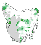
Using what you’ve learned about the Tasmania dataset and mapping with geopandas, reproduce this selection frequency map. To practice your mapping skills, make the map look as similar to this one as possible. Specifically:
Planning units that were already protected should be clearly distinguishable from all others. (Recall: they have a
'status'of2in pu.dat.)The outline of Tasmania should be visible, but the outlines of planning units should not be.
Your map also needs to show the coordinates (in the reference system of the provided shapefiles), have a meaningful title, a legend (colorbar), and be saved as a high-resolution version (≥150 dpi, 8 x 6 inches).
A few suggestions:
pandasoffers two functions for joining DataFrames and GeoDataFrames on columns:joinandmerge. They are similar, but their usage is slightly different. Either will work for you.joinjoins on indices by default. The easiest way to join two DataFrames or GeoDataFrames is to give both the correct index (withset_index()), and then join them withdf = df1.join(df2).mergejoins on columns by default. You have to provide column names as arguments. If the column names are identical, you can pass the name as the argumenton, otherwise, you need to pass the two column names asleft_onandright_on:
df = df1.merge(df2, left_on='planning_unit', right_on='pu_id')
Recall that you can plot any subselection of a
GeoDataFrame(select rows, thenplot). This is useful when you want to apply different color schemes to different subsets of polygons (e.g. for planning units that are already protected).To plot all polygons of a GeoDataFrame with the same color, call the
plotfunction without a variable name, and add the argumentcolor.coloraccepts colors in a wide variety of formats: single-letter codes ('c'), hex strings ('#4adfcf'), a tuple of RGB values (0-1) ((0.5, 0.5, 1)), or legal html names ('lightgrey'). Try out this last one. Does it look like a color you can find on the map?The shaded color map of the map above does not exist as a default colormap in Python. However, you can reproduce it:
from matplotlib.colors import LinearSegmentedColormap

CMAP_DICT = {
    'red': [(0.0, 1.0, 1.0), (1.0, 0.0, 0.0)],
    'green': [(0.0, 1.0, 1.0), (1.0, 0.6, 0.6)],
    'blue': [(0.0, 1.0, 1.0), (1.0, 0.2, 0.2)],
}

my_cmap = LinearSegmentedColormap('', CMAP_DICT)
This colormap can be passed to any plotting function that accepts a
cmap(cmap=my_cmap).
Tip
Understanding the CMAP_DICT code block (optional) allows you to create any color gradient:
CMAP_DICT is a dictionary that contains, for each base color used in additive color mixing ('red', 'green', 'blue'), a list of positions (stops) on the color gradient.
Each position contains a tuple of three values:
position on the gradient (value between
0.0-1.0)intensity of base color before the position (value between
0.0-1.0)intensity of base color after the position (value between
0.0-1.0)
In other words, the dictionary is interpreted as follows:
For
red, start at the beginning of the color scale (position0.0) with 100% intensity (1.0), then move to the end of the color scale (position1.0), gradually reducingredintensity to 0% (0.0). Repeat for green and blue, but with different end values. The resulting RGB values at the beginning of the gradient will be white ((1.0, 1.0, 1.0)), and the final RGB values will be(0.0, 0.6, 0.2)– which represent the color of the darkest green in the above map.
For more information, check out the reference page for LinearSegmentedColormap.
2.1.6. Wrap up#
Does your map look like the map above? Great!
Don’t forget a title, coordinates, and the legend for the selection frequency (e.g., the default colorbar).
Save the high-resolution version in your class folder as:
~/ee508/reports/lab2/1_selection_frequency_tasmania.png
Submit the file to the assignment on Blackboard, and you are done!
2.1.7. Appendix#
Here are two little helper functions to help you skip ahead.
2.1.7.1. run_marxan#
You can run Marxan from Jupyter with this function. It accepts the filepath of the Marxan project, runs Marxan in that folder (assuming that the Marxan executable is already in the project folder), and prints outputs below the cell.
def run_marxan(dir_marxan, silent=False):
    """Run Marxan

    Parameters
    ----------
    dir_marxan : str or pathlib.Path
        Root directory of Marxan project (with data and executable)
    silent : bool
        If False, prints all Marxan outputs.
        Set to True to silence outputs when running lots of jobs.
    """
    import os
    import platform
    import subprocess

    # Pick the correct executable for OSX and chip
    if platform.system() == 'Darwin':
        if platform.processor() == 'i386':
            marxan_command = './marxan_osx10_x86'
        elif platform.processor() == 'arm':
            marxan_command = './marxan_osx11_m1'
    elif platform.system() == 'Windows':
        marxan_command = 'Marxan_x64.exe'
    elif platform.system() == 'Linux':
        marxan_command = 'Marxan_x64'

    # Change into Marxan folder
    os.chdir(dir_marxan)

    # Run Marxan
    if silent:
        proc = subprocess.Popen(
            marxan_command,
            stdout=subprocess.DEVNULL,
            stderr=subprocess.DEVNULL,
        )
        proc.wait()
    else:
        # Run with output printed under Jupyter cell
        proc = subprocess.Popen(
            marxan_command,
            stdout=subprocess.PIPE,
            stderr=subprocess.STDOUT,
            text=True,
        )
        for line in proc.stdout:
            print(line, end='')

        proc.wait()

# Usage example
run_marxan(DIR_TASMANIA)
2.1.7.2. change_marxan_parameters#
You can change Marxan parameters with this function. It accepts the path to the parameter file input.dat and a dictionary of parameters with new values.
def change_marxan_parameters(path, change_dict):
    """
    Function to change the parameters in a Marxan parameter file

    Parameters
    ----------
    path : pathlib.Path
        Complete path of the parameter file ('input.dat')
    change_dict : dict
        Dictionary of parameter values to be changed
        Example: {'BLM': 0.1, 'NUMREPS': 100}
    """

    import os
    import re

    # Check if configuration file exists
    if not path.exists():
        print(path, 'not found')

    # Read configuration file
    with open(path) as file:
        old_text = file.read()

    # Copy the text, keep the old one
    new_text = old_text

    # Loop through each dictionary item
    for key, value in change_dict.items():
        # Define REGEX search pattern string
        search_regex = '\n' + key.upper() + ' +[0-9A-Za-z. -]+\n'

        # If the parameter can be found, print warning and skip to next item
        if re.search(search_regex, new_text) is None:
            print('Parameter ' + key + ' not found')
            continue

        # Define replacement string
        if type(value) == float and value < 0.001:
            value = '{0:.10f}'.format(value)
        replace_str = '\n' + key.upper() + ' ' + str(value) + '\n'

        # Replace strings
        new_text = re.sub(search_regex, replace_str, new_text)

    # If a change has been made, write the file
    if new_text != old_text:
        with open(path, 'w') as file:
            file.write(new_text)
            print('Saved new parameters to ' + path.parts[-1])