2.3. Improving the plan: cost proxy and planning units
Model results are often dependent on modeling assumptions and underlying data. Here we will explore the implications of different assumptions by repeating the above exercise with different inputs. If you have the code ready to go from your last deliverable, the following modifications should not take a lot of coding time (although they will definitely take some processing time).
Deliverables
Two additional selection frequency maps for Colombia:
Municipalities as planning units, heterogeneous cost (estimate based on travel time to cities).
Hexagons as planning units, heterogeneous cost (estimate based on travel time to cities).
An executive summary of your Marxan analysis for Colombia.
Due date
Friday, Oct 17, 2025, by 6:00 p.m.
2.3.1. Include a cost proxy
So far, we assumed that the cost of protecting a hectare of land is constant across Colombia. This is obviously not true. A property in the suburbs of Bogotá or Medellin will have a very different land value than a property in the middle of the Amazon.
Although there is no good land cost layer for Colombia, we can approximate at least some of the heterogeneity in land costs by using a travel time proxy.
We will use a global raster map of estimated travel time to major cities. Its methodology is documented in Weiss et al (2018). You can find a version of the dataset, clipped to the extent of Colombia, in:
The links to the global layer in the above article don’t seem to work anymore. If you’d like to work with the global data for your project, you can find it at:
Use zonal stats to extract the mean travel time for every municipality.
Note
The travel time raster has a “nodata” value of -2147483648 and a “water” value of -9999.
You have to make sure these values don’t make it into your calculation of the mean travel time. Otherwise, you get counter-intuitive numbers (negative travel times).
Use rasterstats.zonal_stats with the argument nodata=-9999 to remove the water pixels. Although that also overwrites (and thus omits) the raster’s other nodata value (-2147483648), you won’t notice, because those values don’t overlap with our planning unit.
If you prefer to use rasterized zonal stats instead, make sure to exclude (mask out) pixels with nodata / water values from both rasters before computing mean travel times for planning units.
Use pandas to compute a new cost column with the following formula, where area is given in square kilometers (recall you already computed a km2 column).
Recall that the operator for raising a value to a specific power in Python is
**. Alternatively,pandasSeries have apow()function that serves the same purpose.If you used rasterized zonal stats to compute the average travel time, you might get infinite cost values (for urban cores with zero travel time). Unfortunately, infinite values break Marxan. As as simple hack, you can overwrite the infinite values with the maximum of the finite cost values (so these planning units stay expensive, but don’t break Marxan).
is_inf = mun['cost'].eq(np.inf)
mun.loc[is_inf, 'cost'] = mun[~is_inf]['cost'].max()
Re-run the parts of the code that need to be updated.
Find a good BLM that allows you to see how patterns change near cities.
You can find a dataset of Colombia’s cities (point geometries) at:
~/ee508/data/external/lab2/colombia_cities.gpkg
The data comes from a NaturalEarth cities dataset, circa 2018. It contains Colombias cities and towns sorted by descending population size. The absolute numbers seem outdated, but the ranking is fine. To see only big cities, you can pick the first 5 with
.head(5)or.iloc[:5]before plotting. Consider scaling the points by population size.
Save a high-resolution version of the resulting selection frequency map. Give it a meaningful title that includes the BLM.
~/ee508/reports/lab2/3_selection_frequency_colombia_traveltime.png
question
How does the map differ from the previous map? Why do you think that is the case?
If you are not sure, plotting a map of the travel time raster or the planning unit cost proxy will likely help you in the interpretation of the differences.
2.3.2. Change the planning unit
So far, we made the assumption that protection decisions are made at the level of the municipality, i.e. a municipality is either protected or not. However, in most circumstances, protection choices are more fine-scale. How do results change if we change the planning unit to a smaller grid?
We will use a hexagonal grid of Colombia, which you can find at:
In creating this grid, I chose a cell size that results in 1110 planning units, so the processing time is approximately in the same range as in the previous exercise. You can run analyses at a finer spatial grain, but they will take longer.
Reproduce the results from Lab 2.2 using the hexagon layer instead of the municipality layer.
You might want to use a new subfolder so you don’t overwrite your municipality-level results:
~/ee508/data/processed/lab2/colombia_hexagons
Use the same travel time cost proxy. Use rasterstats.zonal_stats with all_touched=True for the travel time extraction. You don’t need to simplify the polygons, as hexagons are already simple.
Do not use rasterized zonal stats or all_touched=False to obtain the travel time. A few of the hexagons slivers are very small and will not get a travel time value assigned otherwise. Empty or infinite values in the cost column will break Marxan.
Note that you still need to calculate the hexagon areas, amounts of species range in each hexagon, and boundaries between them.
Find a good BLM.
Save a high-resolution version of the selection frequency map. Give it a meaningful title that includes the BLM.
~/ee508/reports/lab2/3_selection_frequency_colombia_hexagons.png
question
How does the map differ from the previous map? Why do you think that is the case?
Inspiration might come from the parts of the map that contain species with very small ranges inside the study area.
2.3.3. Write up an executive summary
Imagine having to explain the essence of your analysis and your findings to a small audience of colleagues, journalists, or policy makers (pick one group or any combination of them).
Assume they have no knowledge of systematic conservation planning or Marxan. You can assume that they know Colombia and understand species ranges. Write up a short summary (600-800 words), answering the following questions:
What precisely does the analysis do (goal and process)?
In a few sentences, cover:
What is the “structure” of the decision problem that Marxan solves?
How is “optimality” defined?
How does Marxan search for near-optimal solutions? (not more than a sentence)
What do selection frequencies mean? How are selection frequencies different from (near-)optimal solutions?
Important
Make sure you understand why the selection of high-frequency planning units is not guaranteed to give us a network that achieves all species range targets.
How do the three maps differ from each other, and why?
Why do all of these maps identify locations that are different from (additional to) those we saw highlighted in the maps of weighted species range richness from Lab 1.4? After all, we’re using exactly the same species distribution rasters.
Finally: what is one modification to the framing, data, or methods that a researcher (you?) could implement to make this analysis more useful for real-life decisions?
Feel free to add figures, as appropriate. Save it as:
~/ee508/reports/lab2/3_executive_summary.docx
Tip
Avoid the following common mistakes:
Implying that selection frequency and optimal solution are the same concept.
Implying that species richness and species representation are the same concept.
Stating that high-cost areas are never selected into a Marxan solution.
Stating that a given BLM value always implies the same degree of clustering (e.g., when comparing analyses with very different cost data ranges/distributions).
Being vague about the context in which you use the word “optimal” or “optimizing”. The intended meaning of these words can range from extremely specific (e.g., if the decision problem is precisely framed) to extremely broad (e.g., in many everyday contexts).
If it’s not clear why these items are errors, revise Section 1.1 - 1.8 of the Marxan manual.
2.3.4. Wrap up
Submit the following three files as a .zip archive to the Blackboard assignment:
3_selection_frequency_colombia_traveltime.png3_selection_frequency_colombia_hexagons.png3_executive_summary.docx
Nice job!
You just ran your first systematic conservation planning exercise in Marxan, complete with robustness checks of underlying assumptions, and delivered a report with potential relevance for a policy maker.
2.3.5. Did you like this exercise?
If you liked this exercise in complementarity-based conservation planning, Marxan-style, now is a good time to think about whether you want to base your project on this lab.
Question
Is your problem a complementarity-based (minimum set) problem?
Not every problem is - so not everything needs Marxan. But if you think about conservation “features” broadly as anything you want to preserve a minimum quantity of, and that overlap with other features - e.g., ecosystems, views around certain iconic spots, culturally important locations - there are many possible extensions to the minimum set problem.
Some starting points for project ideas:
Is there an assumption in this lab that you did not like?
What happens if you relax it - or introduce a better assumption?
How do results change if you use the Libro Rojo data from Lab 1-5 Option 2 instead?
A new Biomodelos dataset with >8,000 species is now available. How do your results change if you look at thousands of species?
Servers are down sometimes (e.g. Oct 10, 2025)
Explore conservation planning case studies using Marxan around the world.
https://marxansolutions.org/community
If you find one that interests you, perhaps you can request access to their Marxan dataset and enhance their analysis?
Given that planning unit seems to matter: would you like to conduct a parcel-level analysis in a U.S. state, e.g., as part of the Group project?
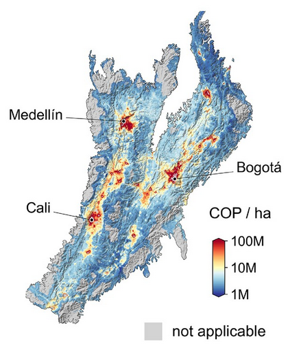
In 2023, we published our own estimates of conservation costs in the Colombian Andes region, based on data from ~2000 public land acquisitions. Does the “better” cost data affect the priorities at all?
The training data, cost raster, and code are on Dryad (public). The cost estimate doesn’t cover all of Colombia, but you can restrict your planning units to the Colombian Andes.
(The paper also does a Marxan-style conservation planning exercise.)
Are you interested in conservation planning anywhere else in the world?
In the United States, this dataset is waiting to get an update:
Again, the paper contains a Marxan-style conservation planning exercise for the United States, courtesy of Josh Lawler et al. The Marxan dataset is downloadable.
A new opportunity cost layer just dropped for Europe. Do you want to use public IUCN species range data to propose a pan-European plan?